How to Prevent Future Accidents of Autonomous Driving
During my time at Volkswagen research, I set up car fleets for sampling training data for autonomous driving. In the end, the outcome was that it is nearly impossible to sample enough training data initially to prevent accidents on the road - as sadly proven by Tesla’s autopilot in the last months (see here and here).
To overcome this problem, a system has to be created where cars, regardless of their brand, sample their environment during operation and ”dangerous“ situations are detected by a central server and propagated to other cars in real-time. This blog post explains how such a system can be realized and how its requirements can be fulfilled, that is, operating in real-time and detecting „dangerous“ situations, what I term anomalies. This blog post explains for the first time how autonomous driving can be linked to website monitoring.
What are dangerous situations?
Imagine your are on your way to work. Today, you are on a divided highway. It's a sunny morning and you are looking forward to the barbecue with your wife tonight. What a great day. You turn the autopilot on as you did it 1,000 times before. You read the newspaper and relax. Now it happens: It's a divided highway and a tractor trailer on the opposite lance decides to turn left in front of you. You have enough time to break but you read an article about the upcoming elections. Your car doesn't notice the white side of the tractor trailer against a brightly lit sky due to the rising sun, so the brake is not applied. You crash into the tractor trailer.
This was exactly the setting of the Tesla accident, where the 45-year-old Joshua Brown was killed when his Tesla Model S went under the trailer of an 18-wheel semi and the roof of his car was torn off by the impact.
These "dangerous" situations have to be detected in order to prevent such accidents.
What we can learn from website monitoring?
Tesla calculated that their fleet has to drive 10 billion kilometers to train and calibrate their machine learning algorithms to drive autonomously. The challenge for autonomous driving, however, is that the algorithms can hardly be trained initially with all possible driving conditions. This is caused by the highly dynamic run-time environment for the sensors, due, for example, to different weather conditions. Thereby, dangerous situations, or what I call anomalies, only occur at a very low frequency. This problem cannot be solved by increasing the amount of training data, since there will be driving situations where no data will be available due to disturbed or noisy sensor output. Therefore, you don’t need more data but a monitoring system able to detect regions where the probability is high that sensors will fail.
This is very similar to the challenge my team and I are currently facing at Sevenval. Over the last two years, we’ve developed the big data analytics product wao.io for website monitoring by processing high volumes of web log data in real-time. We sample page views and correlate them with load times and error rates to analyze the customer experience on websites. We do this to prevent down times of websites (also called anomalies), since the better the availability and customer experiences are, the higher the revenues for online shops or publishers such as newspapers. In summary, website monitoring is the process of testing and verifying that end-users can interact with a website or web application as expected. Website monitoring is often used by businesses to ensure website uptime, performance, and functionality are as expected. This is exactly what is needed for autonomous driving. We want a system that ensures optimal performance and functionality as expected. Let’s have a closer look at website monitoring to learn how we can leverage it for autonomous driving.
At Sevenval, we want to deliver the best customer experience to all mobile customers regardless of the mobile device, operating system or browser they use. That is, we suffer from the same highly dynamic run-time environment and have to optimize the website code to all possible combinations of mobile devices, operating systems and browsers. Since the number of different devices, released versions of browsers and operating systems continues to proliferate, we cannot test them beforehand. Device manufacturers such as Samsung or Apple release updates without announcing them beforehand and giving us the opportunity to test them with customers’ webshops. So, we have to monitor the performance during run-time (when it is too late) and fix them as soon as possible to minimize the damage, that is, the losses of revenue due to bad customer experience.
Monitoring automotive data
In the automotive industry, the need for monitoring comes from sensors that deliver highly dynamic output for the machine learning algorithms. Car manufactures have to produce and sell their cars for profit. This is usually achieved by scaling out production, since the car industry is a very price-sensitive market. Tesla, for example, is still not profitable. Elon Musk’s first master plan said that profit would come when Tesla starts producing and selling a high-volume, lowest-cost model as planned with the Tesla 3 for this year. Lowest-cost also means, however, using lowest-cost sensors such as cameras. Cameras and deep neural networks are currently the gold standard for autonomous driving (see my last blog post). NVIDIA, for example, released this video some months ago showing how a car can be trained to drive autonomously by using cameras and training neural networks with the massive power of NVIDIA’s GPUs. So, car manufacturers have to use image sensors on the one hand to get all details of their environment and scaling out their production but on the other hand have to handle a critical shortcoming, specifically their highly dynamic output.
Image data is precisely the source of the problem and its associated dynamics come from. Image sensors deliver highly dynamic output, that is, colors and frequencies of recognized objects. Areas, such as faces of buildings for example, are low frequencies in image data. Corners and edges of such objects, for instance, add the high frequencies to the image data. And these high frequencies are the important part of the data which machine-learning algorithms need to operate best. This is very similar to how the human’s eye works when we drive a car. We sample our environment through our eyes, browse for objects (meaning high frequencies) to avoid collisions and follow the right direction, measure the distance to the objects by making a stereoscopic projection and deciding what to do next based on all of this information. We are able to drive despite various lighting conditions, for example, at night, at day, through an alley of trees with diffuse light and so on. But what do you see at night, when it is very dark? Less than during the day which means less objects and so less high frequencies. And what do you see when you are blinded by the sun? Usually you see nothing but a white spot, which means more low frequencies and so less high frequencies. In both cases, the lighting conditions eliminate the high frequencies which the algorithms need to work. These high dynamics in the image data are exactly the reason why there will always be situations where the algorithms will fail. Nature is infinite in this case. And that is why a system is needed to detect these ”dangerous“ situations (where the algorithms will fail) with minimal latency and inform other cars which may enter this region.
This is very similar to our problem at Sevenval: the changing lighting conditions correspond to the new releases of browsers, operating systems and devices, which create “dangerous” situations, that is revenue losses for our customers. We call them anomalies, since they occur at low frequency, and use so-called “business events” to detect them. In the next section, I’ll describe how we can use this concept to detect “dangerous” situations in automotive image data.
Detecting anomalies in automotive data
In any case, not all anomalies are bad per se. Usually they are interesting outliers that should be studied for patterns to get a better understanding of your system. Here I provide a brief overview of how we detect anomalies at Sevenval. We monitor our customers’ websites on several different layers in order to discover them. We started with the traditional server monitoring, since we assumed that if the servers run well, the applications on them also run well. Nevertheless, this wasn’t always true. If the “checkout” button does not work on an online shop website, you won’t detect this by server monitoring. This is also true for autonomous driving. Server monitoring would correspond to sensor monitoring. All sensors may work, but if the machine learning algorithms don’t run due to a memory leak or anything else, you won’t detect this by looking whether the sensors are on or off.
So in the next step, we started monitoring applications, believing that if the application runs well, customers would have a good experience. Nevertheless, that didn’t always follow, either. The application may run but if a customer has to wait longer than 10 to 15 seconds for a page, there are studies that show that there is a high probability for leaving the website. In the case of autonomous driving, the machine learning algorithms may work. If they take too long, however, to analyze the sensor data or the sensor data is noisy, the car will make the wrong decisions while driving. Noise could be induced, for example, if the camera is blinded by the sun or occluded. So, you have to measure that, too. And that is why we need what I term “business events” which measure on the highest level of abstraction if our system works or not.
To adequately monitor customers’ websites, we decided to measure the website’s load time in the browser, that is the time until the customer can interact with the website. This metric gives us direct feedback regarding how well the entire application works and covering the most important part of business, the point of sale. This is why we measure all of our metrics in the browser, using such customer clicks and so on. If these metrics drop suddenly, we know that there is something bad going on. When a user is able to interact with the website, we say the customer can see the relevant website and trigger page view events. Basically, a page view is a view by a customer, which was our first business event next to the load time. The counterpart for autonomous driving would be the number of autonomous drives. If we count, for example, the number of trips in a specific area at a specific time and we see that this number decreases suddenly, we can assume that there is something going on why the cars are not able any more to drive autonomously.
The next metric that we measure is the website’s load time. If the load time increases, we can assume that the servers are either not able to handle the current number of customers or the application suffers from an outage, for example, because the database is down. The load time is an important quality factor.
So what could be a similarly important quality factor for autonomous driving?If I imagine that I were driven autonomously to work every morning, I’d be happier on days when I arrive at work without having lost time in a traffic jam. This lost time is directly reflected by the average cruising speed. So, cruising speed is definitely an important quality factor for autonomous driving. If we detect a drop in case of the cruising speed in a specific area, there could be a traffic jam, roadwork or rough weather conditions (such as black ice) forcing the cars to slow down.
Another metric that we sample is the number of customers’ mouse and keyboard clicks. If this count drops, we know that the website may be negatively impacted, since this is the fundamental way visitors interact with a website. Regarding autonomous driving, which is massively based on data from image sensors and computer vision algorithms, this metric could be the number of detected objects per second, since this metric is fundamental. If you see then, that this metric drops in a specific area or on a specific road, you can assume that it is difficult to drive autonomously in this area. This could stem from rough lighting conditions, visual occlusions due to roadwork and so on. Once this is detected by system and a specific geographic region is labeled anomalous, this can be propagated to other cars, which are about to enter that region, since there will be a high likelihood that the cars have to switch into “manual” mode and be controlled by a human driver.
Now that we’ve defined the metrics that we want to sample in each car, in the next section we can review a system that is able to receive such events from a group of cars and analyze them in real-time to inform other cars about anomalies (real-time is required, since, for instance, one second of blind driving on a highway by a speed of 100km/h, corresponds to 50 meters of blind driving per second).
How to set up real-time architectures for autonomous driving
In order to understand real-time (often called stream) processing, we first have to compare it to batch processing. Batch processing is the gold standard in business intelligence and the natural first resort for processing data. Batch processing means processing data in chunks: first collecting, then ingesting and finally processing the data in batches. It is a very efficient technique for processing high volumes of data with excellent accuracy. How long it takes to process the data is not important. Batch jobs are configured to run without manual intervention and process the entire dataset. Depending on the amount of the data being processed and the computational power of the system, batch processing may delay the output significantly. When time is not an issue, batch processing is a very mature and easy-to-set-up technique.
In contrast, stream processing involves continuously ingesting, processing and outputting data. It emphasizes the velocity of the data. Data must be processed incredibly quickly, nearly in real time. Stream processing gives decision makers the ability to adjust for contingencies based on events and trends developing in real-time. This is exactly what we need to detect anomalies for autonomous driving.
In order to realize batch and stream processing for big data applications, a standardized architecture was designed and very widely used: the Lambda architecture. In 2014, a new type of architecture emerged, which was termed Kappa architecture, which specializes in the needs of stream processing. The Lambda architecture suffers from some pitfalls for stream processing. To understand the shortcomings of the Lambda architecture and the differences between the two, let's first examine what the Lambda architecture looks like:
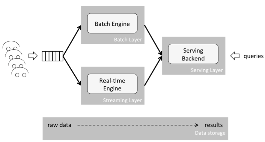
As depicted above, the Lambda architecture consists of three layers: a batch layer, a speed (or streaming) layer, and a serving layer. Both the batch and streaming layer receive a copy of new events, in parallel. The serving layer then aggregates and merges computation results from both layers into one answer. The batch layer (also termed the historical layer) has two major tasks: managing historical data and re-computing results such as machine learning models. Computations are based on iterating over the entire historical data set. Since the data set can be very large (tera or peta bytes of data), this produces accurate results at the cost of high delays, or latencies, due to long-running computations.
The speed (or streaming) layer provides low-latency results in near real-time fashion. It performs updates using incremental algorithms, thus significantly reducing computation costs, often at the expense of accuracy.
Let’s look at an example of its implementation. At my current job, for example, we analyze huge amounts of web logs to detect bad load times, and present this data in a dashboard. Regarding the load time, we compute the median value. To calculate this value, all load times have to be sorted and the value has to be found, where 50 percent of the rest is above and below this value. Due to sorting the data, this computation is quite expensive from the computational perspective and requires the accuracy of the entire data set. To enable our clients to flexibly and quickly analyze any time period, we analyze data in chunks of hours and days and sum up the results to match the time period of interest. Since analyzing an entire day is very time-consuming, we do this in the batch layer once a night. The speed (or streaming) layer analyzes the last hour of the current day and computes its median value. The results are merged in the serving layer, where the median values of all sub time periods, that is the contained days and hours of today, are considered and weighted according to their portion of the entire time period. Weighting time periods in this manner to calculate the overall median value leads to inaccuracies, since the accurate value can only be achieved by sorting all values of the entire time period and not only the already aggregated ones. Nevertheless, our method quickly assesses any desired time periods, at the expense of lower accuracies. In terms of autonomous driving the cruising speed in specific regions could be computed by the same procedure, however, with the same inaccuracies.
Simply put, the Kappa architecture is a Lambda architecture without a batch layer. To understand how this works, let’s have a closer look at what batch processing fundamentally is. A batch is a set of data with a start and end time; hence it is a “bounded” piece of data. On the other hand, a stream is “unbounded”, meaning it is not constrained by a start or end time —it is infinite. That is why a batch can be interpreted as bounded stream, which is a subset of stream processing. Based on this conclusion the Lambda architecture can be simplified to a single streaming engine, the Kappa architecture, which is able to handle both batch and real-time processing. Another benefit is that the overall system complexity is reduced significantly as presented in the figure below:

To sum it up, the main benefits of the Kappa architecture are:
-
Everything is a stream: Batch operations are a subset of streaming operations. Therefore, everything can be treated as a stream.
-
Less code duplication: A single analytics engine is required and not two, in contrast to the Lambda architecture. Code, maintenance, and upgrades are easier and code duplication is reduced.
-
Reprocessing by replaying: A state can always be re-computed as the initial record is never changed. Computations and results can be re-produced by replaying the historical data from a stream. The data pipeline must guarantee that events stay in order from generation to ingestion. This is critical to ensure consistent results, as this guarantees deterministic computation results. Running the same data twice through a computation must produce the same result.
To leverage the above benefits the analytics pipeline must be set up in a specific way to allow for storing the raw data and producing results by feeding in this data, in real-time or after the fact. We’ll look at this in the following section. But the Kappa architecture is exactly what we need to fulfill our requirement of real-time processing for autonomous driving. Based on this architecture, we should be able to receive massive amounts of data and analyze it in real-time to detect anomalies.
Setting up the analytics pipeline
Now let’s start building the analytics pipeline. First, we identify the components which are required. After putting a component in place to handle thousands of parallel connections from our cars sending their data to our backend, we need a scalable, distributed messaging system with events ordering and at-least-once delivery guarantees. A distributed message queue such as Kafka is able to wire the output of one process to the input of another via a publish-subscribe mechanism. Based on this, we can build something similar to the Unix pipe system where the output produced by one command is the input of the next.
The second component is a scalable stream analytics engine. Inspired by the Google Dataflow paper, Flink, at its core, is a streaming dataflow engine that provides data distribution, communication, and fault tolerance for distributed computations over data streams. One of its most interesting features allows one to use the event timestamp to build time windows for computations. Alternatively, we could use Spark in streaming mode instead of Flink. Both are good choices, but we’ll go with Flink here.
The third and fourth components are a real-time analytics database. We’ll use Elasticsearch combined with Kibana, a powerful visualization tool. Those two components are not critical, but they’re useful to store, display and query raw data as well as results. This is important to work with the data to get new ideas and to understand how and why the machine learning algorithms came to their results.
Based on the aforementioned components, the analytics pipeline could be implemented as depicted in the following figure:
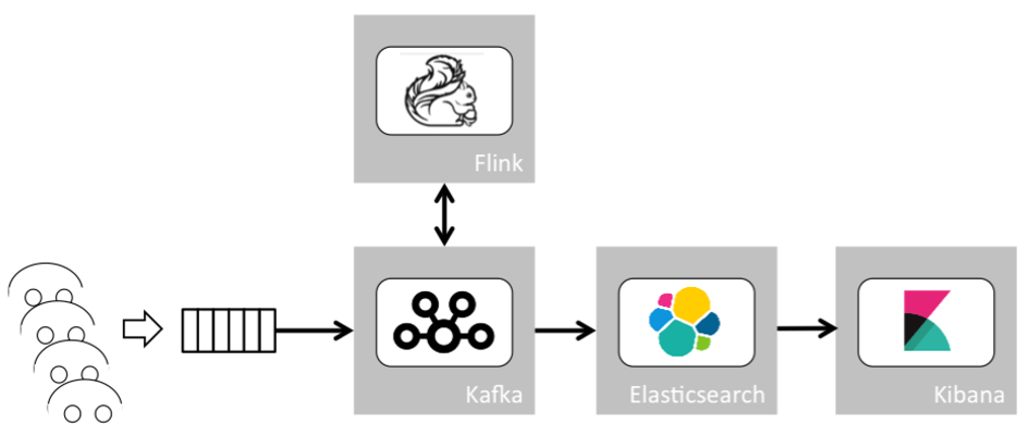
This pipeline consists of several micro services where outputs of services can be reused and wired to other services. Each micro service can thereby be assigned to a simple, well-defined scope. This micro service architecture paves the way for fast development of new features. Additionally, data ordering and delivery are guaranteed, allowing for high data consistency. Last but not least, event timestamps can be utilized to build timeframes for computations.
In the context of autonomous driving, each vehicle sends its data to our gateway. Optimized gateways and appliances based on the MQ telemetry transport protocol (short MQTT) could be used in order to handle thousands of vehicles and concurrent connections. Then the data is sent to Kafka. Kafka wires this data to distinct Flink (or Spark) jobs which do the pre-processing and the final processing. With this powerful data pipeline in hand, let’s examine how a statistical model can be implemented to detect dangerous situations (or anomalies) for autonomous driving.
A model for anomaly detection for autonomous driving
In this section, we consider autonomous driving as a system, which consists of cars in a specific place at a specific time. In order to detect anomalies in such a system, meaning detect situations where the machine learning algorithms will not be able to drive the passenger safely, we use a statistical model to analyze the aforementioned business events in that geographic region and time period. I published a paper at the 25th World Wide Web conference in Montreal this year for detecting such anomalies in web log data. In both contexts, anomalies are defined as unpredictable and dangerous situations that are very different from previous observations. My model utilizes dynamic base lining and creates a multi-dimensional target space based on an initial data set. This data may stem from test drives (perhaps based on “clean” training data that the machine learning algorithms used to learn) or from live data from a car fleet. It is important that this data comes from the geographic region and the type of cars in the monitored system. Additionally, dynamic base lining can be used to fine-tune the target space during run-time. Based on real-time data from vehicles, the current overall system’s state is located in the target space.
Now let’s look at how we construct the target space and do live monitoring. The history of the system is split at some point in time, ts, in a target-space and a current part, hT and hC, respectively, as depicted in the following figure. The drives in time period hT are used to calibrate the target space of the application for the combined metric μ, illustrated by the colored areas. The current location of the application in the target space is determined based on the drives in hC. Based on this data, we compute the metric μ, which indicates whether an anomaly has to be reported or not. As an example, let’s consider a case where the sun blinds the cars’ image sensors in a specific region and the image sensors are no longer able to detect objects. The number of detected objects would drop in this region. Thereby, μ drops which triggers an anomaly in our model and detector.
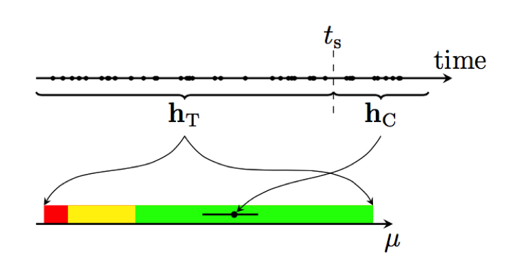
Now let’s deep dive in how the target space and μ are computed. The target space is defined by generating bootstrap samples from hT. Bootstrap is a non-parametric method for statistical inference, which is not restricted by initial assumptions. Thereby, we can take any metrics for building our target space without knowing their distributions before. Having these samples allows us to calculate confidence intervals for each metric, for example, the cruising speed, the number of detected objects by image sensors and so on. Since the used metrics are uni-directional, i.e., the smaller or larger the better, we can restrict ourselves to single-sided confidence intervals. These are given by the appropriate quantiles of the metric samples and define the target space regions. Similar to the ApDex, which is the gold standard for web monitoring, we define three different regions. We consider the current state of our application as normal, if all metrics are within the best-95 % range (i.e., the 95 % confidence interval). The state is defined as“frustrating” if any of the metrics is in the worst-5 % (worst-1 %) range, where the frustrating state takes precedence.
Accordingly, we define the combined metric for the current history, hC , μ. μ is computed for all pre-defined geographic regions by taking the maximum of the probabilities to find a better value than the observed one for each metric. This metric can be interpreted similarly to the p-value of a sample, i.e., the smaller the observed μ, the larger is the difference between the sample and the target-space history. The following table lists the target space regions and the associated μ intervals.
| Region | Confidence interval | μ range |
|---|---|---|
| Normal | Best 95% | 1.00 – .05 |
| Tolerating | Worst 5% | .05 - .01 |
| Frustrating | Worst 1% | .01 – 0 |
The overall data pipeline, combining the transformations mentioned before, will look like this:
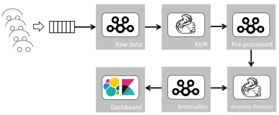
This data pipeline receives the raw data, extracts statistical information (such as cruising speed or number of detected objects by the image sensors per car), applies our model over the interesting business events (statistical and raw), and outputs anomalies whenever they are found.
How might cars respond to anomalies?
When I discussed my idea of such a monitoring system with colleagues in the past, they often asked me: „And how might other cars respond to certain anomalies?“ The answer I always gave was: Like a white blood cell that has observed a virus/bacteria and tries to bring your body back to homeostasis.
This means that autonomous cars could respond to anomalies by re-calculating their routes and choosing paths where no anomalies have been detected. This would probably be the easiest reaction.
Conclusion
In this blog post, I’ve presented an approach to setting up a monitoring system for autonomous driving. Dangerous situations – or so called anomalies – can be detected in specific geographic areas in real-time. This information can be propagated to other cars to inform them and prevent them from trying to drive autonomously, although there is a high probability of not being able to. In order to build such a system I introduced the Kappa architecture for real-time processing of big data sets and a self-training (online) statistical model able to yield quick, accurate analytics.


